In essence, a nanoLC system consists of the same components as a standard HPLC system. However the reduction of the column i.d. has the consequence that all components of the LC instrument, including injector, pump, tubing and detector must be downscaled according to the downscale factor. Successful operation of nanoLC, achieving the maximum efficiency, is only possible if the extra-column peak broadening is kept small in comparison to the peak volume. Employing a 75 µm i.d. nanoLC column typical peak volumes are in the range of 80-150 nl. These peak elution volumes indicate the necessity for strong miniaturization of all components of the LC system.

The mobile-phase flow rate in nanoLC is in the range of 10-1000 nL/min and can be generated by standard HPLC pumps applying flow splitting or by dedicated splitless pumps. Both types of pumps are able to deliver solvent gradients in the nanoliter per minute range reliably. Splitless pumps have the advantage that less solvent is consumed. Standard pumps with a flow splitter can deliver a wide flow rate range and generally have a lower gradient delay time.
The performance of a nanoLC pump is determined by the accuracy and precision of gradient formation, flow delivery and the mixing efficiency. A significant improvement in flow rate accuracy and precision has been achieved by the incorporation of liquid flow sensors capable of measuring flow rates down to several nl/min. Current nanoLC pumps are capable of delivering solvent gradient at 50 nl/min with a precision better than 0.2% RSD. 

NanoLC gradient performance
The performance of a nanoLC gradient pump is determined by the gradient precision, gradient accuracy and gradient delay time.

• The gradient precision directly influences the retention time precision and is therefore a very important specification of the nanoLC pump. The gradient precision can be measured experimentally by performing repetitive solvent gradients. Addition of a UV absorbing compound, e.g. acetone, to one of the solvents, allows to record the gradient profile. An overlay of the UV traces will indicate the precision of the gradient formation. Another well accepted method for the measurement of gradient precision is to perform consecutive gradient separations of peptides. The retention behaviour of peptides is strongly dependent on the solvent composition. The variance in the retention times of the peptides expressed in %RSD is a measure for the gradient precision. 

Overlay of peptide separation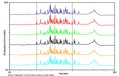NanoLC separation of bovine serum albumin tryptic digest Column: 15 cm x 75 µm i.d. PepMap C18, 3 µm Flow rate: 300 nl/min Mobile phase: A) water, 0.05% TFA B) acetonitrile/water (80:20 v/v), 0.04% TFA Gradients: 4-55% B in 30 min, 5 min wash at 90%B, 15 min at 4%B UV detection: 214 nm, 3 nl flow cell Injected amount: 1 pmol

• The gradient accuracy is influenced by the proportioning of the solvents and by the dispersion of the gradient in the nanoLC system. The gradient accuracy can be measured by generating a step gradient profile with a UV tracer added to one of the solvents. Deviation of the experimental step gradient profile from the programmed gradient indicates a difference of the mobile phase composition. Differences in the height of the gradient steps indicate inaccurate proportioning of the solvent, rounding of the steps indicate dispersion in the system.
• The gradient delay time is dependent on the gradient delay volume and flow rate of the mobile phase. In a nanoLC system that uses flow splitting the gradient delay time is determined by a pre- and post split component. The gradient delay time can be directly determined from the difference between the programmed and experimental step- or linear gradient.

The maximum injection volume that can be made on a column without causing dispersion is directly proportional to the column volume. Injectors with internal loop sizes as small as 4 nl are currently available, but the precise alignment of the small port boring and the extremely narrow loop groove is challenging. Another disadvantage is that the injection volume can only be changed by replacement of the rotor seal. Split loop injection can be applied with internal loop injectors with larger loop sizes but suffers from inaccurate and imprecise injection performance.
In discussing sample injection techniques for nanoLC it is important to distinguish between solute focusing and non-solute focusing conditions. Under these conditions the injection volume is very critical and must be reduced according to the down-scaling factor.

Many of these limitations can be circumvented by applying solute focusing during sample injection. Solute focusing, click to download Power Point animation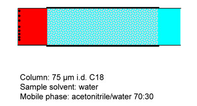Blue: mobile phase in C18 column;
Orange: sample solvent;
Black spots represent sample components with high retention factors.

The sample is dissolved in a solvent with lower elution strength compared to the mobile phase. After injection the analytes, depicted as black dots in the animation, are transported through tubing to the column in the sample solvent (red phase). Upon reaching the column the analytes are focused or concentrated onto the head of the column as a result of their high retention factors. Solute focusing allows that much larger sample volumes can be injected. Next, the elution strength is increased to elute the analytes (not shown).

The principle of solute focusing is widely applied in nanoLC analysis of peptides. Most peptides are readily dissolved in aqueous solutions and are eluted from the reversed-phase column with an acetonitrile water gradient. A common technique in which solute focusing is applied for large volume injections in nanoLC is column switching.
The heart of the column switching set-up is a 2 position switching valve. This valve ‘connects’ the trap column with the nanoLC separation column. The experimental set-up for column switching in nanoLC is shown below.

Microcolumn switching (Downloadable PPT file)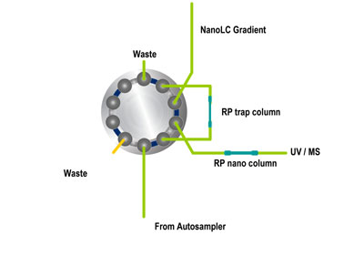

Steps in micro column switching:

1. Sample injection by autosampler onto RP trap column with highly aqueous solvent
2. Sample preconcentration takes place due to extremely high retention factors
3. Valve switching to place trap column in series with RP nano column
4. NanoLC solvent gradient started to elute compounds from RP column
5. Detection by UV and/or MS
6. Valve switching to prepare for next injection (not shown)

In micro column switching the sample is injected onto a small trap column. The trap column has a low flow resistance, a small volume and a high sample capacity. The stationary phase is similar as that of the separation column. A second, isocratic pump is used to transport the sample to the trap column. The low flow resistance of the trap column allows the use of high flow rates to inject large sample volumes in a short time.

The column switching has the advantage that, by concentrating the sample onto the trap column, conventional size injection volumes can be made on 75 µm i.d. nanoscale LC. In addition this set-up can be used for various on-line sample clean-up strategies, e.g. desalting of samples on C18 columns.

Almost all commonly applied detectors in HPLC have been miniaturized for use in nanoLC. To avoid dispersion during detection the volume of the flow cell must be adapted to the size of the peak volumes eluting from the column. Ideally, the maximum detection volume should be not more that 10% of the volume of the peak. Consequently, for analytes eluting from a 75 µm i.d. nanoscale column having peak volumes of around 50 nl the maximum detection volume is 5 nl only. The effect of the detection cell volume on the peak width is shown below. The extra column dispersion using the relatively large 45 nl UV flow cell is clearly seen by the decrease of resolution between the peptides.

Effect of flow cell volume on separation of tryptic peptides of cytochrome c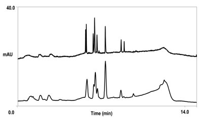Figure 7 Effect of flow cell volume on separation of tryptic peptides of cytochrome c  in a 200 µm i.d. monolithic column in capillary LC. Upper chromatogram detection cell 45 nl, lower chromatogram 3 nl. Flow rate 2.5 ul/min, detection 214 nm.
 
Using UV detection the sensitivity is proportional to the path length of the flow cell according to Lambert-Beers law. Significant improvements in detection sensitivity can be achieved by extending the path length using specially Z- or U- shaped UV flow cells. These flow cells are made of fused silica and can have an effective illuminated path length of 10-30 mm.
 
 
Coupling to MS
NanoLC can easily be coupled to mass spectrometric detectors. The reduced flow rate of nanoLC facilitates solvent evaporation that is required in the coupling to MS. Both on-line LC-MS coupling via electrospray ionisation (ESI) and off-line coupling via matrix assisted laser desorption ionisation (MALDI) are standard techniques.
The nanoLC-ESI interface is formed by a spray needle having a diameter of approximately 20 µm and a tip of around 5 µm. The electrospray is started by applying an electric field between the needle tip and MS. During the electrospray process the solvent is evaporated and compounds are ionized. The reduced flow rate yields smaller droplets by which the ionization efficiency and sensitivity are enhanced.
For the coupling of nanoLC to MALDI-MS the mobile phase is fractionated onto a MALDI plate by micro fraction collector. Solute compounds that are eluted in the mobile phase are post column mixed with matrix solution that is required for MALDI ionisation. Depending on the average peak width the fraction collection time is adjusted. After solvent evaporation and crystallisation of the matrix the MALDI plates can be transferred to the MS for analysis. The coupling of nanoLC to ESI- and MALDI-MS is schematically illustrated below. 

Schematic of nanoLC-ESI-MS (Click to download Power Point animation)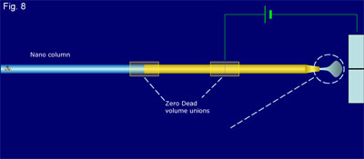Steps in nanoLC-ESI-MS:

1. Sample components are separated onto the nano column and reach the nanospray needle tip
2. Electrospraying of mobile phase results in small droplets
3. Mobile phase solvent is evaporated and charge causes Coulombic repulsion.
4. The charge density on the surface causes the droplets to disrupts. The process is repeated until gas phase ions are left.
5. Charged sample compounds enter MS
6. Sample compounds are detected by MS

Schematic of nano LC Maldi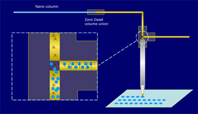Steps in nanoLC-MALDI-MS:

1. Mobile phase with dissolved sample components is mixed with MALDI matrix solution in zero-dead volume T-piece
2. Solvent is leaving the system through needle
3. MALDI target is moved after predefined time intervals to collect mobile phase in discrete fractions
4. MALDI target is transferred to MALDI MS instrument for detection

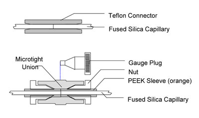
The choice of connecting tubing and connectors is an important consideration in nanoLC. In particular tubing and connectors placed post-column, where no solute focusing is possible, need to be selected properly to avoid additional peak dispersion. Dispersion in cylindrical tubing is described by the Aris-Taylor equation and increases to the power of four with the internal diameter of the tubing. Typically fused silica tubing with an internal diameter of 20µm is used for connection of a 75 µm i.d. nanoLC column to the detector (UV cell or MS orifice). Zero-dead volume connections of fused silica tubing can be made with a piece of tefzel tubing or with a stainless steel or PEEK union. These union types of connections can withstand high backpressure and can also be used for pre-columns.

Types of connectors for fused silica tubing and columns (low pressure, high pressure)